LCD dynamics
Intro
On this page, several aspects regarding the response timing of LCDs will be explained and discussed. It is assumed that the reader is familiar with the basic working principle of LCDs, like the screen being comprised of a pixel matrix, a pixel being divided into sub-pixels for the primary colors, a sub-pixel cell being filled with liquid crystal fluid and acting like a light valve without actually emitting light by itself, and a light source sitting behind the pixel matrix in form of a backlight which we assume here to be made of white LEDs.
The figures shown here often contain illustrations of time functions that could be measured with a fast photo-diode. It should be kept in mind, though, that the human visual system does not necessarily work that fast and, therefore, is not really up for perceiving all the details that can be technically measured. On the other hand, the visual system can be incredibly sensitive to all kinds of effects. Moreover, there is quite a natural variance in how sensitive individuals are, let alone the variance coming from individual experience (e.g., gamers versus non-gamers). In short, one should be careful in drawing conclusions from these time functions about what a stimulus would look like to a human observer.
Pixel response


At the left hand side of the figure, a temporal sequence of 4 frames is shown which represents the screen content at 4 subsequent time points while a white rectangle is moved rightward by some number of pixels per frame. The green circle just marks a fixed position on the screen. Pixels at this position will undergo a black-white-black transition as the rectangle is moved over this fixed position. The green dotted curve ("input") in the according time plot at the right hand side of the figure illustrates the ideal pixel response where the pixels switch instantly back and forth, which would result in the white rectangle being displayed with sharp left and right edges. However, because the pixel response is sluggish (red time course, "response"), the rectangle would actually look more like the one shown on the frame at the bottom of the figure (corresponding to the 3rd frame in the frame sequence), where the pink dotted outline marks the intended rectangle position; however, the right "edge" of the rectangle is not quite as white as it should be, and the background beside its left edge is not quite as black as it should be, thereby forming a t(r)ail.
This type of figure (Figure 1) is used throughout this page and illustrates the optical transmission state of a liquid crystal cell (aka pixel – or sub-pixel, to be precise) over time. The vertical lines mark the start of the LC panel update cycles and provide an absolute time reference. The y axis can be interpreted either as the optical transmission state or, if a continuously active backlight is assumed, as the relative pixel luminance. In either case, the valid range goes from 0% (cell "closed") to 100% (cell "open"). The green dotted curve ("input") depicts the intended time course of the pixel state as sent by the LCD controller to the panel after a corresponding pixel value was received from the PC's graphics card. The red solid curve ("response") depicts the pixel response, that is, how the pixel's optical transmission state (or luminance) changes over time.
If the cell is "open", light coming from the back (i.e., the backlight) can pass through the cell, making the pixel appear bright. If, on the other hand, the cell is "closed", backlight is blocked and the pixel appears dark. For the time being, pixel color will not be taken into account, so "bright" can be used synonymously for "white".
A sluggish pixel response is usually not observed directly, because the human visual system is sluggish as well and bad at picking up absolute errors. For example, if an object would appear suddenly, just out of the blue, we couldn't tell whether it appeared really instantly (that is, within nanoseconds) or whether it appeared rather slowly (that is, within milliseconds), at least we couldn't tell without a direct side-by-side comparison. However, as soon as motion comes into play, which allows temporal aspects to be translated into the spatial domain, effects caused by a sluggish pixel response can become much more apparent. Figure 2 illustrates how the rendering of moving edges would require pixels to be switched instantly and how a non-ideal pixel response affects the actual display of the edges of a moving object in the spatial domain. Pixels at or near the edges will appear as a mix of background and foreground color, here resulting in gray, which can be picked up rather easily because the true foreground and background colors can be observed right next to the edge pixels for direct comparison.
Obviously, a sluggish pixel response will cause artifacts, but how these artifacts exactly look like depends on several factors like the velocity of the object, the refresh rate, and the sluggishness of the pixel response (the response time, for short). If, for example, the response time is in the order of one refresh cycle and the object velocity is high enough for the object to be displaced by several pixels per refresh cycle, the object would look like it was followed by its own copy, a more or less transparent ghost. On the other end of the artifact spectrum, where the response time is rater long in comparison to one refresh cycle and where the object displacement per refresh cycle is small, the object would look blurred along its motion trajectory. So depending on the relative magnitude of the determining factors, the artifact can be anything between ghost images and blurred edges.
Note that this kind of edge blurring is different from the edge blurring that can be observed when following the object with the eyes. The latter is often more prominent because the blurred edges appear more likely close to the visual focus, where we pay more attention and have a higher spatial resolution than in the periphery. Moreover, edges of objects which are followed by the eye also appear to be stable, meaning they are not moving with respect to the visual focus, making any edge oddities more easily observable and accordingly more disturbing. The two types of edge blurring are also different in how strongly they depend on the frame rate. While the blurring that is induced by eye movements becomes weaker at higher refresh rates, the blurring induced by a sluggish pixel response might just appear differently (smooth blur profile versus more distinct ghost images, as explained above).
Figure 2 illustrates what happens at a physical level and, thus, what would be measured. But how would such motion stimulus actually look like, given that our visual system is sluggish as well? In fact, what has been described here for the screen pixels should also be happening at the photoreceptor level on the retina, where sluggish photreceptors play the same role as sluggish pixels, even if the stimulus was presented with absolute perfection like, for example, when looking at a moving object in the real world. However, the visual system has its own ways of dealing with its own sluggishness, but these ways are fine-tuned to the very properties of the visual system and are optimized for delivering an as veridical percept of the real world as possible. Any blur that actually originates from the outside world should ideally be perceived "as is", that is as a blur. So it should not come as a surprise that we would perceive artificially caused blur as blur while, at the same time, our visual system is perfectly capable of compensating for the blur that originates from the sluggishness of the photoreceptors and the visual system itself. Anyway, in how far the pixel-response-induced artifacts described above, be it ghost images or blurred edges, are of practical relevance depends on how strong other artifacts are in comparison, for example, the above-mentioned eye-movement-induced motion blur.
Incomplete pixel update
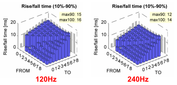
Each pixel cell has its own small electrical circuit which receives pixel voltage updates from the panel driver and maintains the pixel voltage throughout the pixel's refresh cycle. This circuit is hooked up to the panel driver only once per refresh cycle and only for a very short time. It is only during this short time when the panel driver can actually change or "refresh" the voltage of the particular pixel. The small circuit acts like a sample&hold device, sampling the possibly new voltage level and then holding this voltage until the next refresh. But neither the sampling nor the holding works perfectly; the hold stage, for example, might be leaking, in which case the term "refresh" takes a literal meaning. Or the voltage update corresponding to a big pixel value change might be incomplete, so that actually more than one refresh cycle is needed for completing a change, as illustrated in Figure 3. This update effect might have other explanations (see side note below), but whatever the explanation is, the effect somewhat slows down the pixel response. Whether an increased refresh rate helps to alleviate this problem depends on whether or in how far the underlying cause becomes more relevant at higher refresh rates. Measurements made with the BenQ XL2540 suggest that going from 120 Hz to 240 Hz, for example, indeed reduces response times, although not dramatically (see Settling curves of the BenQ XL2540). This is also reflected by slightly improved rise and fall time measurements for 240 Hz (Figure 4).
Side note: The observed incomplete update could also be explained by the dielectric properties of the cell which change as the liquid crystal molecules are aligning with the electric field. The LC cell can be seen as a capacitor which is charged (or discharged) to the target voltage. During the refresh cycle, the liquid crystal molecules align – slowly but surely – with the electric field, thereby also changing the dielectric coefficient and, accordingly, the electrical capacitance (C) of the cell. Provided that the charge (Q) is not changing (meaning, no current is flowing into or out from the capacitor, because the local pixel circuit is disconnected from the driver), it is the voltage (U) that has to change (Q=U·C). If there was no further voltage refresh, the cell would finally settle at an accordingly wrong voltage, resulting in an accordingly wrong pixel luminance. However, at the beginning of the next refresh cycle, the voltage will be refreshed to the original input value, thereby re-accelerating the switching process, which results in these small bumps in the luminance curve. The fact that the incomplete update is observed for small as well as for big voltage changes speaks for this explanation and against the theory of the driver circuit being just too weak.
Default (no-voltage) cell state
The cell state (open vs. close) depends on the spatial orientation of the liquid crystal molecules in the cell, and this orientation depends on the mechanical and electrical forces the liquid crystal molecules are exposed to. Technically, the cell state is modulated by applying a voltage to the cell. When no voltage is applied, the molecules in the cell are exposed to only mechanical forces which pull the molecules into one orientation, corresponding to the cell being in one state, lets say the "closed" state. Whereas when a voltage is applied, the according electrical field overruns the mechanical forces and pushes the molecules into a different orientation, corresponding to the cell being in the other state, lets say the "open" state.
Importantly, the "open" and "closed" states are kind of end states, meaning that the cell can neither be driven beyond "open" by applying more voltage, nor can it be driven beyond "closed" by applying less than no voltage. While "less than no voltage" is physically impossible anyway – at least here, where negative voltages will have the same effect as accordingly positive voltages (see the Pixel inversion section) – "more voltage" is actually well possible. This gives rise to a potential asymmetry in how fast transitions between any two cell states can be made, depending on the direction of the state changes. Usually, the transitions toward the voltage-driven state (so here, toward the "open" state) can be made faster than transitions toward the "no voltage" state, although there are physical limits and technical constraints as of how far this can go, that is, how much faster the voltage-driven transition can be made. It also depends on how strong the mechanical forces are in comparison to the electrical field which has to overrun these forces. Whether the possibility of boosting the voltage beyond the cell's saturation level is actually being used by manufactures is questionable (see Accelerated pixel update (overdrive) section for evidence).
Whether the "no voltage" condition corresponds to the "open" or the "closed" state is actually a technical choice, and pixel response timing is only one of several criteria to be taken into account. Apparently, also the panel type plays an important role in this respect, given that most TN panels are "normally white" (that is, "no voltage" corresponds to "open"), whereas other panel types, like IPS or VA panels, are usually "normally black".
Please note that for a "normally white" panel, a low voltage corresponds to high luminance and vice versa, which can create some confusion when associating voltages with luminance (in the figures shown on this page, for example). That is why we assume panels to be "normally black" throughout this page (so rather according to IPS or VA panels), unless otherwise mentioned.
Accelerated pixel update (overdrive)

The top panel shows the pixel response curve (blue solid line) for switching to a target level (green fat-dotted line). The blue dashed line is the response curve according to some hypothetical overdrive target level (green dashed line). This overdrive level was chosen so that the according response curve intersects the requested target level at the end of the first refresh cycle after the target level change (encircled in red).
The bottom panel shows the pixel response (red solid line) when the hypothetical overdrive level from above is actually applied, but just for the first cycle after the switch; thereafter, the original target level is applied (green fat-dotted line).
Overdrive is a method of accelerating the pixel response by applying higher than normal voltage changes in response to changed pixel values. The voltages are set back to normal after usually one refresh cycle, where "normal" refers to whatever levels are needed for the settled states, corresponding to the respective nominal pixel values. Figure 5 illustrates a case of "optimal" overdrive – "optimal" in the sense of making the pixel response as fast as possible without provoking any overshoot. Not provoking overshoot is just one of many possible optimization criteria though. One could argue, for example, that some overshoot can be tolerated as long as it is too weak and/or too fast for the visual system to be picked up. Obviously, technical constraints have to be taken into account as well, and even more criteria come in to play when considering factors like, for example, color and strobed backlight (see the according sections below).

Note that overdrive can be applied in both directions, that is, "higher than normal voltage changes" can result either in voltage boosts (when switching from dark to bright) or in additional reduction of voltages (when switching from bright to dark). If overdrive is supposed to work for all nominal pixel voltages (where "nominal" refers to voltages that correspond to the settled pixel states), some headroom has to be made available at both ends of the voltage range. When thinking in terms of luminance, this demand for headroom would require allocating part of the available luminance range just for overdrive, thereby reducing the visible luminance range accordingly. This, however, would come with a loss in contrast, more so for clipping off headroom at the low end of the luminance range than clipping off headroom at the high end. This asymmetry is due to the fact that making black a bit brighter has far more impact on contrast than making white a bit darker. Unfortunately, compensating for such contrast reduction by just boosting the backlight is of no help, because contrast is generally independent of the maximum backlight level – a brighter backlight not only makes white brighter but also black, while the ratio of the two, i.e. the contrast, stays the same.
When thinking in terms of voltages instead of luminance, the asymmetry already mentioned in the Default (no-voltage) cell state section comes into play. The subtle difference between luminance and voltage in this context is that, although making headroom at the "no voltage" end of the voltage range is impossible without cutting into the nominal range – same as with luminance –, making headroom at the high end can be achieved by further increasing the voltage without actually changing the according optical transmission state – if the LC cell is already fully open at some voltage, an even higher and beyond-saturation voltage cannot open the cell any further, but the higher voltage can still accelerate the process of opening. This provides the opportunity of making headroom at the low luminance end without having to sacrifice luminance range where it is most precious (contrast-wise). However, this requires the panel to be of the "normally white" type (like TN panels), where the saturation voltage end falls at the low end of the luminance range. In this case, that is when using beyond-saturation voltages for boosting switches towards the low luminance end, making headroom at the high luminance end is only possible by cutting into the visible luminance range, which is a smaller pill to swallow than having it the other way around. Well, so far for the theory of how to use beyond-saturation voltages for overdrive. In practice, beyond-saturation voltages actually seem not to be used to any measurable extent, at least not as part of the user-settable overdrive mechanism; if it would be used, we should observe a benefit for switches of type any-to-black (or any-to-0 in terms of pixel values) when overdrive is activated, which we don't. It still could be though, that beyond-saturation voltages are used in any case, that is irrespective of the user's overdrive setting. But given that it is actually not so trivial to implement this without crushing the lower end of the pixel value range, beyond-saturation voltages are probably not used at all. This also means that there is no substantial difference, as far as this aspect of overdrive is concerned, between "normally black" (IPS, VA) and "normally white" (TN) panels. The limiting factor is always the non-overdriven any-to-black switching times, which – coincidentally or not – happen to be smaller than the non-overdriven any-to-white switching times, irrespective of panel type. Because of this timing asymmetry, overdrive is not only good for speeding up pixel response times but also for making switching times more equal across all the switching possibilities (i.e., any-to-any, without having to cut into the luminance range at the "wrong" end). Having equal switching times becomes the more important the slower the pixel responses are (see also the section Pixel response asymmetries and color).
What about the timing of overdrive? The time points for applying or removing overdrive voltages is bound to the regular pixel refresh cycle. Currently, probably most overdrive implementations apply overdrive voltage only during one refresh cycle after a pixel value change. Shorter refresh cycles, i.e., higher refresh rates, allow for, but also require more aggressive overdrive for it to be effective. For example, in case of the optimal overdrive criterion that was used for Figure 5, the final state is supposed to be reached after one refresh cycle, irrespective of the duration of the refresh cycle. This, however, assumes that there are unlimited overdrive resources available, which is obviously not the case in practice. Figure 6 illustrates the difference regarding overdrive requirements for two different refresh rates. Overdrive, at least if implemented equally well for all pixel levels, always costs something, be it in terms of contrast or in terms of other factors, as explained above. Evidently, limitations regarding overdrive headroom affect any-to-black and any-to-white luminance changes first, whereas any-to-gray changes are increasingly less demanding the closer the gray comes to the 50% gray. So the higher the refresh rate the more overdrive headroom is needed for maintaining a certain overdrive effect, at least if overdrive is applied for only one refresh cycle. Just to emphasize this, if the refresh rate is increased without making more headroom available for overdrive, it is not only that overdrive does not get any better with the higher refresh rate, it is even that overdrive gets worse – up to a point where it basically does not make any difference anymore whether overdrive is applied or not. Although a lack of headroom can be partially compensated by applying overdrive for more than one refresh cycle, the necessity of doing so would also mean that the effective pixel response time, that is, the overdrive-boosted response time, is considerably longer than one refresh cycle, thereby compromising the benefits of having higher refresh rates in the first place. Extending overdrive to more than one refresh cycle also makes overdrive calculations more complicated, at least when doing it right. Although multi-refresh-overdrive is certainly doable, it might not be worth the effort. Luckily, higher refresh rates help reducing the pixel response time even without overdrive, as mentioned in the Incomplete pixel update section. This can compensate, at least to some extent, for overdrive becoming less effective at higher refresh rates.
Screen update
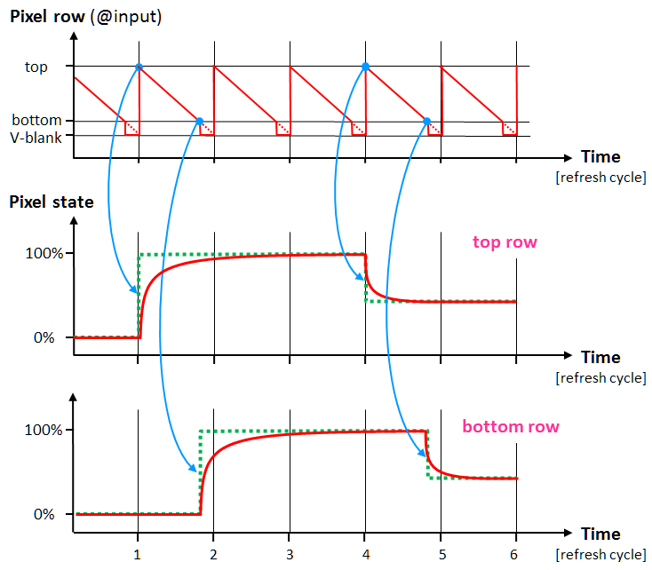
Top curve: Y location (i.e., pixel row index) over time of the pixel data as it is received at the monitor's video input (i.e., as sent by the PC's graphics card). Note that the curve is not depicting the pixel data but only the screen location the received pixel data refers to, over time. "V-blank" is just a virtual location used here to indicate the pause interval between receiving the last visible row of the current frame and the first row of the next frame.
Mid curve: Response curve of a pixel at the screen's top row for a hypothetical pixel change from dark to bright and, after 3 refresh cycles, back to a mid level.
Bottom curve: Response curve of a pixel at the screen's bottom row, which is exactly the same curve as for the top row but shifted in time, according to the later reception of the according pixel data.
What has been discussed so far only concerned the response of single pixels but without taking into account that the pixels are not updated all at the same time across the panel. The panel (or pixel array), is usually updated in a sequential order, from the top of the screen to the bottom. The update timing is ultimately controlled by the monitor controller, the so-called scaler, but the timing often closely follows the timing of the video signal as it is received from the PC. Because of the sequential panel update, the top pixel row is changed/updated at the beginning of the panel update cycle, whereas the bottom pixel row is changed/updated shortly before the end of the panel update cycle (see Figure 7). It is only "shortly before", because there is a more or less small pause – the vertical blanking interval (VBL) –, which was chosen here to mark the end of the panel update cycle (it is a matter of definition though which event marks which part of the update cycle). Importantly, the pixel responses look the same at each screen location, except for the time shift that reflects the different update times within the panel update cycle, as illustrated in Figure 7.
Strobed backlight
Backlight strobing, that is, turning the backlight on once per refresh cycle and for only a short period of time, is a method of reducing motion blur. It is actually the two types of motion blur mentioned earlier already, which are reduced, – the pixel-response-induced and the eye-movement-induced motion blur. The pixel-response-induced motion blur has been explained in detail in the Pixel response section already, so here just a very short explanation of the eye-movement-induced motion blur.
When presenting a moving object on the screen, it can be displaced only once per monitor refresh cycle, so the object motion is more a stop-and-go rather than a smooth motion, and, importantly, the object is always visible while stopping (assuming the backlight is permanently on). On the other hand, when following this object with the eyes, the eyes follow smoothly – hence, smooth pursuit eye movements –, which makes the stop-and-go-displayed object appear moving rapidly back and forth on the retina, one back-and-forth cycle per refresh cycle. This repeated back-and-forth motion is too fast for the visual system to be seen as motion. Instead, the back-and-forth motion is smashed into a blur – the motion blur. This is similar to the blur in a photograph that was taken with a camera in shaky hands, and an exposure long enough for capturing a good part of the shaking (assuming the camera not having an image stabilizer).
The motion blur can be reduced by making use of the stroboscopic effect, thereby hiding the object for the most part of its back-and-forth movement on the retina. This is accomplished by switching the backlight on for only brief periods of time (the strobes) and only once per refresh cycle. This does not only reduce eye-movement-induced motion blur but can also reduce pixel-response-induced artifacts, provided that the strobe timing is such that the strobes do only "highlight" the pixels when they have sufficiently well settled. Unfortunately, when it comes to the technical realization of backlight strobing, the interplay between backlight strobing and sluggish pixel response is so troublesome – as will be explained in the following – that backlight strobing probably would not be worth it, if it was just for reducing pixel-response-induced artifacts. In other words, strobed backlight is used primarily for reducing eye-movement-induced motion blur.
Note that strobed backlight must not be confused with pulse width modulated backlight (PWM backlight). Strobed backlight refers to turning on the backlight only once per refresh cycle and very briefly so, whereas PWM backlight implies the backlight being turned on and off several times per refresh cycle, normally not even synchronized with the refresh cycle at all.
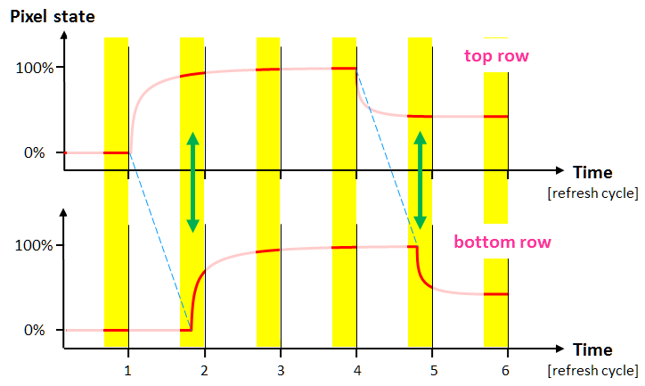
In its simplest form, the backlight can be controlled for only the entire screen, and instantly so (within microseconds). Because the sequential pixel updating process comes with pixel responses that have a different delay with respect to, say, the start of the refresh cycle, depending on the pixel's Y position on the screen, a global backlight strobe pulse makes different parts of the pixel responses visible, as illustrated in Figure 8. While pixels at the top of the screen might have nicely settled already when the strobe "highlights" the screen, pixels at the bottom of the screen might have barely started changing. Under circumstances like the ones shown in the figure, pixels at the top never appear to be in an intermediate state, whereas for pixels at the bottom the intermediate state appears even more pronounced by being literally highlighted. "Intermediate state", in this context, means that old and new image information are mixed, and the extent to which new image information is spoiled by old image information is called cross-talk. As is the case with the sluggish pixel response, also cross-talk becomes most apparent in presence of motion or rapidly changing scenes, and the according artifacts are closely related to the pixel-response-induced artifacts discussed in the section Accelerated pixel update (overdrive). Just to recap, the pixel-response-induced artifacts could be anything between ghost images and blurred edges, depending on object velocity, refresh rate, and response time. Strobing the backlight adds just another factor to the already complicated interplay between those factors. Without going further into detail here, the bottom line is that strobed backlight cannot help with edge blur (meaning the pixel-response-induced edge blur, not the eye-movement-induced motion blur), but it might actually help with ghost images (by reducing cross-talk) – or make it worse (by aggravating cross talk). Furthermore, if the pixel response is sluggish enough to cause more edge blurring than ghosting, not only will cross-talk have little visible effect (despite being strong in a technical sense) but, also, will strobed backlight be of little use for reducing eye-movement-induced motion blur, which, in this situation, will be small anyway in comparison to the pixel-response induced edge blur.
It is difficult to make general statements about the over-all usefulness of strobed backlight, because it all depends. Strobed backlight appears to be beneficial, or at least not useless, if the pixel response is clearly faster than one refresh cycle; it becomes rather useless, if the pixel response is clearly slower than one refresh cycle. If the pixel response is in between it depends very much on the object velocities and edge contrasts at hand, and possibly on personal preference, whether strobed backlight does more good than bad.
Turning the backlight on for only part of the time results in less luminous energy being emitted on average, which is compensated, at least in part, by making the backlight brighter for the short time it is turned on. Another downside of having turned on the backlight for only a small part of the refresh cycle is the potential highlighting of spatio-temporal irregularities in the pixel responses. Real-world response function recordings actually don't look as nice and smooth as illustrated in the figures shown here. Normally, this is not an issue as such irregularities average out when the backlight is turned on all the time. But when it is not, more or less subtle artifacts might appear, possibly even depending on the screen region. One relatively common example for such artifacts being exaggerated with strobed backlight are pixel inversion artifacts (see the Pixel-inversion section).
One downside of strobed backlight is that it induces flicker. This flicker appears even stronger to the observer than the flicker of a CRT (cathode ray tube), because the LCD backlight not only switches on and off instantly (instead of fading in and/or out), but the whole screen area is strobed at once (instead of having a scanning backlight strobe).
For the same reason the stroboscopic effect is good for reducing eye-movement-induced motion blur, it is bad for how static objects appear in presence of smooth or even not so smooth eye movements. It is bad because the retinal image of a static object (or a static scene) is not continuously moving across the retina anymore, as it would with permanent backlight, but it pops up at different locations along the motion trajectory (on the retina), one pop-up per refresh cycle. So the visual system expects a smooth motion trajectory but gets discretely displaced images instead, which can be distracting and tiring, even though this is not necessarily perceived consciously.
In some respects, strobing the backlight is very similar to the black frame insertion technique. For black frame insertion, the refresh frequency is doubled and a black frame is rendered every other refresh cycle. Obviously, the so mimicked backlight strobe is rather long. Note that even though nothing of the pixel response curve is hidden in the dark when using this technique, it still helps avoiding cross-talk, which is for two reasons. Firstly, because the major cross-talk is now always between content and black instead between (old) content and (new) content – okay, also the refresh frequency is twice as high, so not much gained regarding cross-talk, because if the response times in a black-any-black sequence are good enough for resulting in enough luminance at even twice the normal frequency, the response time at the normal frequency should be good enough for keeping cross-talk low. But, secondly, the virtual strobe is not global but is delayed according to the sequential panel update, which allows the same settling time for all pixels before being (virtually) highlighted, irrespective of their Y-position (see also the section Scanning backlight further below). Moreover, the virtual strobe has soft edges (slow rise and fall times) due to the sluggish pixel response, which, together with the scanning nature of the virtual backlight, also helps reducing screen flickering. One downside of black frame insertion is the considerable reduction of contrast. While the black luminance stays the same, with or without black frame insertion, the luminance for the content (e.g. white) is basically cut in half, which results in just half of the contrast as compared to the normal mode without black frame insertion.
Overdrive enhancements

Pixels at the bottom of the screen are updated late in the refresh cycle (dashed and faint vertical lines), and the backlight pulse (yellow, before refresh #2) comes shortly after, way before the pixel state has sufficiently settled to the target level, at least when no overdrive is applied (dashed blue curve). Applying overdrive that does not create any overshoot hardly improves the situation (red dotted curve), whereas aggressive overdrive is much better while only a very small part of the undesirable overshoot is made visible by the next backlight pulse (before refresh #3). This residual overdrive could be zeroed if another cycle of overdrive would be applied, which is what history-based overdrive is about.
With strobed backlight, only part of the pixel response becomes actually visible, and which part it is depends on the Y-position of the pixel (top versus bottom, see Figure 8). As mentioned earlier, the time between a pixel being updated and the backlight being turned on determines how well the pixel state has settled and how much cross-talk between frames there will be. In general, the pixel settling can be somewhat accelerated by using overdrive, thereby also reducing cross-talk. But normally too much overdrive is counterproductive as it causes overshoot. On the other hand, if the overshoot is not visible anyway, because the backlight strobe "highlights" a different phase of the pixel response, overshoot can be well tolerated in favor of a more aggressive overdrive. Figure 9 illustrates how a more aggressive overdrive can improve the situation for pixels near the bottom of the screen, where it is the early phase of the pixel response which is made visible by the backlight pulse, leaving the overshooting part of the pixel response in the dark. Obviously, making overdrive so aggressive also for pixels near the top of the screen is less beneficial but, luckily, also less required, because pixels at the top have anyway much more time to settle before the backlight strobe comes (always provided a pulse timing as shown in the figures here). This means that overdrive should be less aggressive at the top of the screen and more aggressive at the bottom. Such Y-dependent overdrive appears to be implemented in NVIDIA's LightBoost and also in NVIDIA's ULMB (Ultra Low Motion Blur).
Another way of enhancing overdrive, which is useful for continuous as well as for strobed backlight, is to take more than only the last pixel value into account when calculating the next overdrive level. Such history-based or adaptive overdrive basically allows to make overdrive more aggressive for one refresh cycle and actively counteract the overshoot effects during the next refresh cycle. Note that the meaning of the term "adaptive overdrive" is not really well defined. It could as well refer to just an overdrive that has been tuned to the Y-position (see above) or to the currently used frame rate, both of which is far less of a big deal than implementing history-based overdrive. History-based overdrive has probably not been implemented in any consumer product yet and it might never be, because it cannot cure the fundamental problem of overdrive needing some headroom to operate effectively, as explained in the Accelerated pixel update (overdrive) section.
Scanning backlight
As explained above, combining globally strobed backlight with the sequential updating of pixel cells causes cross-talk artifacts to be differently strong depending on the pixel's Y-position. The being "differently strong" part can be solved by strobing the backlight locally and in sync with the pixel updating, thereby providing the maximal settling time to all pixels, and not just, say, the top row of pixels. This is what "scanning backlight" refers to. But implementing a scanning backlight is technically much more challenging and therefore more expensive than implementing just a global backlight. For a scanning backlight, the backlight would ideally be controlled for each pixel line individually, but the vertical resolution of practical implementations of scanning backlight is normally much lower than that, which then might give rise to visible horizontal stripe patterns. As soon as motion comes into play, be it object motion, head or eye motion, or smooth pursuit eye movements, the temporal differences between the horizontal segments can become apparent in the spatial domain. Some of the effects might look like screen tearing, which otherwise is only observed when the screen refresh is not synchronized to the video signal input.
If the monitor has plenty of headroom regarding refresh frequency, a scanning backlight can also be mimicked by the technique of black frame insertion, as explained in the Strobed backlight section.
Input lag
Roughly speaking and as understood here, input lag is the time difference between the monitor receiving a new frame from the PC and this frame becoming actually visible. So this notion of "input lag" associates "input" with the monitor input. Other definitions of input lag associate "input" with user input, in which case the input lag would be the time it takes, for example, for a specific mouse displacement to actually become visible on the screen. Anyway, the following is only about the monitor-induced input lag.
When it comes to quantifying input lag, the numbers depend on the exact definition of the involved time points, which is especially tricky for the "becomes visible" time. The "becomes visible" time usually depends on the screen position (e.g., top vs. center vs. bottom ), the backlight timing (continuous versus strobed backlight, strobe pulse timing), and the luminous energy the visual system has to receive before a new frame can be claimed as to be "visible". "Visible" should not be interpreted like in the context of a detection experiment, where it is about the time required for detecting a white stimulus appearing on a black background, for example. It is rather about realizing a change from one image content to the next, where both images are mixed during the transition and the old image might mask the new image for a while, before the new image becomes dominant.
In the case of continuous backlight, the emitted luminous energy is distributed over the entire refresh cycle, so more time is needed for accumulating a certain amount of luminous energy, in contrast to, for example, a CRT monitor where almost all the luminous energy is emitted immediately after the pixel data has arrived at the monitor's input. And this does not even take into account, that, in a CRT, all the luminous energy carried by the update pulse refers to the new frame only, whereas in an LCD, the pixel settling to the new state is not only slow, but also contaminated by old content. In other words, for the new frame to become visible, not only must the pixels have sufficiently well settled to the new state, but also enough luminous energy belonging to the new state must have been accumulated by the visual system in order to override old content. Of course, the visual system doesn't follow this sequential order and all of the involved processes have smooth transitions that are intermingled, which makes quantifying the perceptually relevant timing very difficult. It should be noted that making all the luminous energy available instantly, like with a CRT, does not mean that the visual system is able to process this energy instantly; but it means that it cannot get any better than that (i.e., better than with a CRT), at least regarding input lag.
At a first glance, using strobed backlight seems to be disadvantageous when it comes to input lag, because it means that emitting the luminous energy is delayed until the pixels have settled, thereby causing potentially more input lag than with continuous backlight. On the other hand, once the luminous energy becomes available via the backlight strobe, basically all the luminous energy "belongs" to the new frame already. Plus, the luminous energy normally distributed across the entire refresh period is delivered in a much shorter time, namely just during the short strobe. The abrupt onset of the backlight might accelerate visual processing of the newly incoming information even further. Obviously, all of this is difficult to quantify, like it is for the continuous backlight case.
In conclusion, one should be very careful when interpreting and comparing input lag measurements by the numbers, because they might not really be representative for the according visual effects.
Accelerated panel update, VT tweak
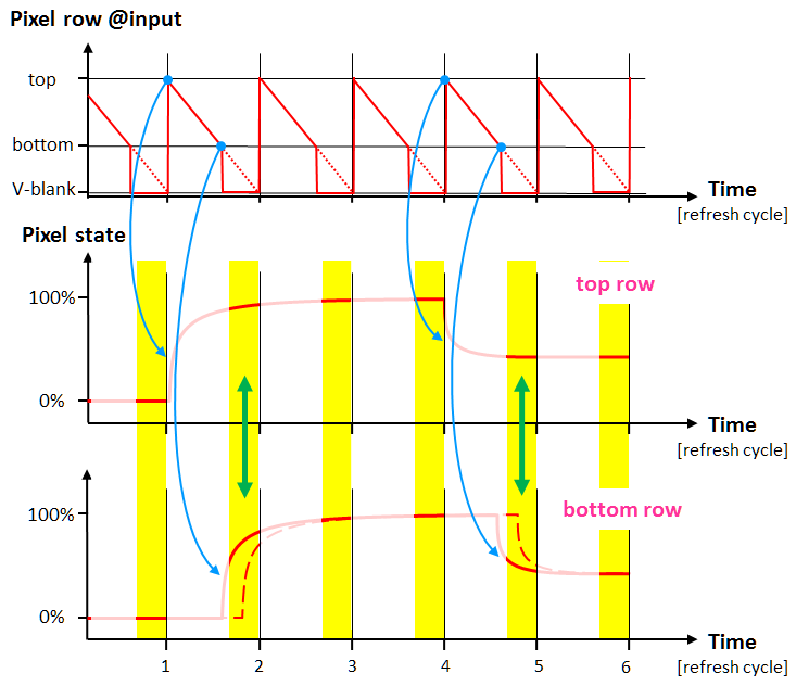
As explained earlier, the panel is updated in a top-down sequence and the update process normally takes almost all of the refresh cycle, followed by only a very short pause – the vertical blanking interval. Technically, however, the update process can be made faster in favor of an accordingly longer pause. With continuous backlight, this will just reduce input lag a bit. With strobed backlight, however, this allows for more settling time before the strobe pulse makes the current pixel states visible; the closer the pixel is located at the bottom of the screen the more settling time is actually gained, as illustrated in Figure 10. Luckily, this is also where more settling time is badly needed.
If the monitor controller (i.e., the scaler) is handing over the pixel data to the panel at basically the same time as it receives the data from the PC, that is, without any further buffering of the data, the update timing is actually determined by the PC's graphics card and can be modified so as to make the vertical blanking interval longer, thereby making the pixel update interval in the monitor shorter without changing the refresh rate. This modification of the graphics card video timing is also called VT tweak, where "VT" stands for Vertical Total, the sum of visible lines plus the lines in the vertical blanking interval. Technically, enforcing a faster panel update is more demanding for the electronics, which might come with downsides like degrading colors, stronger pixel inversion artifacts and alike. A practically feasible upper limit for the update speed can be inferred from the maximum refresh rate that the monitor supports nominally. However, only few models allow tweaking the video timing at all, and even fewer allow to go all the way up to the limit that should be technically possible given the specified maximum refresh rate.
Pixel response asymmetries and color
The color of a pixel is determined by the luminance ratios between the three sub-pixels – red, green, and blue – which make up the pixel. Changing the pixel color usually means that each of the sub-pixels needs to be changed in a different way. One sub-pixel might undergo a switch from dark to bright, the second might not change at all, and the third might change in the opposite way but only a bit. Although the sub-pixel response curves might differ accordingly, the color can still change in a consistent way, that is, the pixel color at each moment in time during the transition can be a mixture of just the old and the new color. However, if things are less ideal, other colors mix in as well along the transition. Even if the color deviates for only a very short time, such color deviations can become quite apparent when motion comes into play, just like the sluggish pixel response becomes apparent in form of blurry edges (Figure 2). For color it is much different in so far as the effect depends on three sluggish response curves and that it is not about the response curves per se but about the ratios between the response curves. While blurry edges cannot be avoided (in moving objects) if pixel responses are sluggish, color shifts can be avoided, meaning that edges in moving objects do not necessarily have to show wrong-colored seams. Such wrong-color seams would be most obvious for monochromatic stimuli with a color mix of at least two primary colors. This includes gray-level stimuli, which are special in so far as the sub-pixel values are always the same, e.g., R/G/B=130/130/130, and they always change in the same way, which should actually be optimal for avoiding any differences in the response curves and thus should not cause any color seams. On the other hand, colors pop out from a gray-level stimulus very easily, so even small color shifts can become quite obvious and distracting. But why would the response curves differ for grey-level stimuli in the first place? Well, they wouldn't, if the R/G/B values were not only equal on the graphics card level but also on the LCD's panel level. But this assumption might actually not be true if the monitor is doing some color management that would imply different gains for the different color channels. In conjunction with non-linearities especially at the lower and upper end of the value range and/or in conjunction with overdrive, R/G/B values at the panel level can be quite different from each other, resulting in accordingly different response curves even for gray-to-gray switches.
Temperature effects
The time constant of the pixel response depends quite a bit on the temperature of the liquid crystal fluid. The fluid is just more viscous when cold, causing the molecules to lose mobility, which then slows down cell response. This is a problem because most if not all of the techniques discussed here have to be fine-tuned to the specific timing of the pixel response. It can be assumed that the fine-tuning (done in the factory) is optimized for a thoroughly warmed-up LCD at otherwise normal room temperature. So best LCD performance can only be expected when the LCD had enough time to warm up. But even then, LC cell temperature might still not be constant, because the pixels cells produce some heat themselves by blocking light – the luminous energy absorbed by a cell has to go somewhere. That is why the cell temperature, and with it the response time behavior, also depends on the content being displayed near by the pixel in question and/or in the proximate past. This effect is small though and usually of no practical relevance.
Pixel-inversion
The open/close state of a (sub-)pixel cell is controlled by a voltage, where the amount of light being blocked by the cell only depends on the absolute voltage but is independent of the voltage polarity. However, the liquid crystal fluid in the cell actually degrades if the mean voltage is different from zero, which is why the voltage polarity has to be inverted at a high enough frequency. In a monitor, the polarity is inverted at the monitor's refresh frequency. It appears to be technically difficult though to meet exactly the same absolute voltage levels at both polarities, even for static image content. Any residual difference in absolute voltages causes an according difference in the cell states and, thus, in pixel luminance. These luminance fluctuations might be perceived as an according pixel flickering at half the refresh frequency. In order to make such flickering less apparent, both polarities are used at the same time but for different sub-pixels, so that potential differences can average out across space (i.e., across adjacent sub-pixels) and over time (i.e., over refresh cycles). Because the pattern of how polarities are distributed across sub-pixels is very regular, pixel-inversion artifacts can still become quite obvious, especially if the temporal averaging is compromised by eye movements of certain velocities, which makes the spatial polarity distribution pattern become more apparent for short periods of time. Pixel-inversion artifacts, or more generally, voltage stability artifacts, can also surface in other forms, like color shifts or cross-talk within pixel rows or columns. These artifacts possibly show up under only very specific circumstances, which makes testing and quantification difficult. Although high pixel densities and high refresh rates both can help in hiding pixel-inversion artifacts, those features also make it technically more challenging to avoid such artifacts in the first place.